Reinforcement Learning with Verifiable Physics: Post-training LLMs with Continuous Rewards
NeurIPS 2026
Massachusetts Institute of Technology
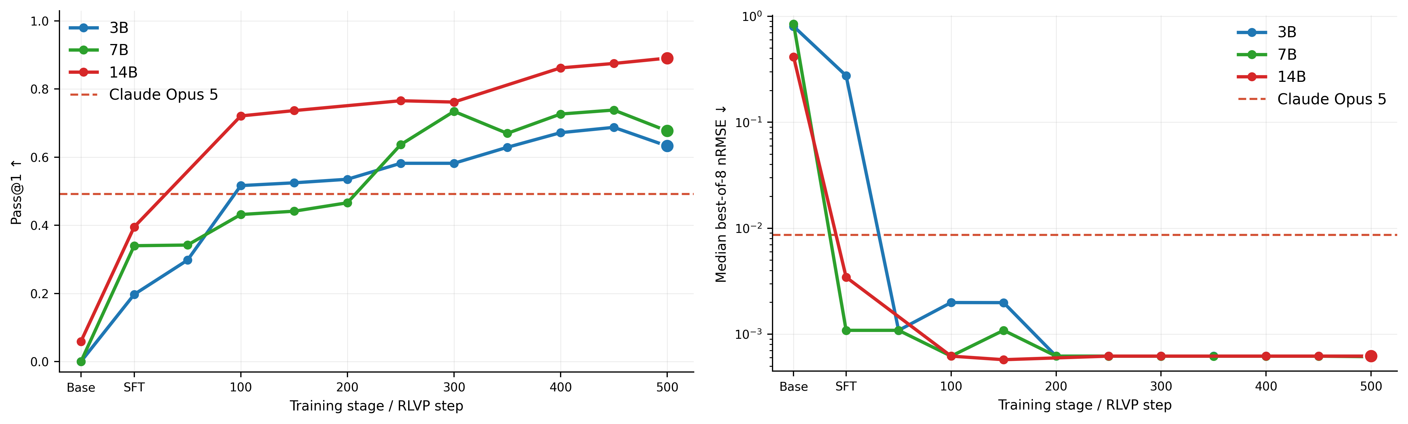
Continuous physics rewards teach LLMs to write more accurate PDE solvers. In our 7B reward ablation, adding physical-accuracy feedback to validity-only RL improves seen-PDE pass@1 from 61% to 76%. Generated programs must pass execution checks; continuous rewards then score the accuracy of their solutions. See the reward ablation below.
TLDR
- RLVP learns from solution error. Programs must run successfully and return valid outputs. Their solutions are then compared with hidden numerical references to compute continuous rewards.
- One model is trained on eight PDE families. We start with supervised fine-tuning on a bank of numerical solvers, then apply GRPO to 3B, 7B, and 14B Qwen2.5-Coder-Instruct models.
- RLVP shows transfer to unseen PDEs. We test ten held-out PDEs and five 3D problems without additional training. Improvements vary across problems.
Abstract
Partial differential equations (PDEs) are foundational to modeling in science and engineering, but constructing reliable numerical solvers remains labor-intensive, demanding expert knowledge of discretization schemes, stability conditions, and boundary treatments. Recent work has begun to frame PDE solving as a code-generation task for large language models (LLMs), yet existing approaches operate primarily at inference time: relying on prompting, debugging, self-refinement, and test-time scaling rather than adapting the model itself. In parallel, reinforcement learning with verifiable rewards has emerged as a powerful post-training paradigm for code and math reasoning, but its verifiers are typically binary: a compiler runs, or a test passes. Such signals discard the graded structure of scientific correctness, where two solvers may both execute and yet differ in solution accuracy by orders of magnitude. In this work, we introduce RLVP: Reinforcement Learning with Verifiable Physics, an RL post-training framework for multi-PDE solver code generation. RLVP addresses this verifiability gap with a hybrid verifier: hard program-validity checks ensure executability, while continuous physics rewards score function-space physical accuracy, with optional PDE-residual consistency. A single policy is post-trained across diverse PDE families spanning hyperbolic, parabolic, elliptic, and incompressible-flow systems. RLVP improves over both pre-trained and supervised-only baselines on the trained PDE families, and shows selective zero-shot transfer to held-out PDEs. Under direct generation, compact RLVP-trained models outperform the evaluated frontier models on the trained PDE families. The trained policy shows evidence of compositionality in numerical motifs: it recombines stencils, time-stepping schemes, and boundary-handling primitives learned from the PDEs used in training into generated solvers for unseen PDE problems.
Method
Continuous physics rewards
We execute each generated solver on hidden PDE instances. Invalid outputs receive zero reward; valid outputs receive a continuous score based on their error against a numerical reference. The accuracy-only reward is
The gate \(V\) checks execution, output shape, and finite values. The temperature \(T_{\mathrm{traj}}\) sets the error scale, and \(\mathcal{L}_{\mathrm{traj}}\) measures normalized solution error:
Here \(\widehat{u}\) is the generated solution and \(u^\star\) is the reference. The norm covers space and time, or space alone for steady-state problems. This gives feedback even when two executable programs would receive the same binary reward.
Full reward formulation
The full reward also includes a PDE-dependent residual factor:
The residual loss penalizes residual excess relative to the numerical reference. Setting \(\lambda_p=0\) recovers the accuracy-only reward above. Each exponential factor can be interpreted as the probability of passing a check with an exponentially distributed error tolerance.
Updating the policy with GRPO
Starting from the SFT policy, we use Group Relative Policy Optimization (GRPO). For each prompt \(x_i\), we sample \(G\) candidate programs, execute them, and compare their verifier rewards. A program's advantage is its reward relative to the group:
Here \(\mu_i\) and \(\sigma_i\) are the group's reward mean and standard deviation. The same advantage is assigned to each response token. GRPO uses these advantages in a clipped policy update, with KL regularization to the frozen SFT reference.
Clipped GRPO objective
For each response token, \(\rho\) is the probability ratio between the current policy and the policy that sampled the program. Define the clipped ratio and surrogate contribution as
The policy maximizes the paper's group- and token-averaged objective:
\(y_{i,g}\) is a sampled program and \(D_{i,g,t}\) is its per-token KL penalty to the frozen SFT policy. The verifier supplies the rewards; no learned value model is needed. See the paper for the token-level definitions and KL estimator.
Results
Why continuous physics rewards matter
An executable program can still return an inaccurate physical solution. Adding a continuous physical-accuracy reward improves the 7B model over validity-only RL: seen-PDE pass@1 rises from 60.9% to 75.5%, and pass@8 from 76.9% to 88.5%. This ablation evaluates 32 generated programs per prompt.
| Training reward | Pass@1 | Pass@8 |
|---|---|---|
| Validity only | 60.9% | 76.9% |
| Validity + continuous physical accuracy | 75.5% | 88.5% |
Pass@k is the estimated probability that at least one of k sampled programs succeeds. Success requires valid execution and normalized solution error (nRMSE) ≤ 0.01. Residual consistency does not further improve aggregate accuracy in this 7B ablation; its effect depends on the PDE and model scale.
Results on PDEs used in training
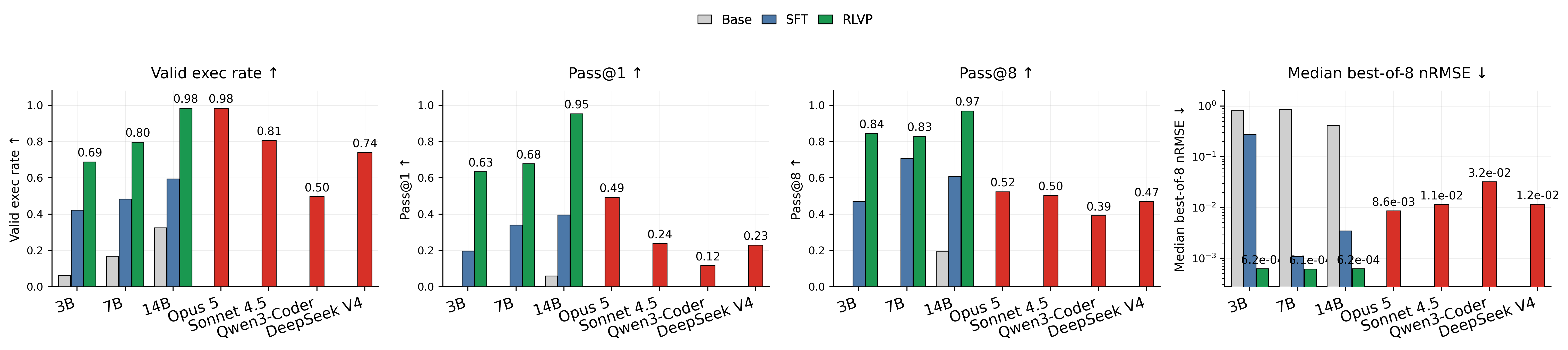
Under direct generation, the full-reward RLVP models outperform the evaluated frontier baselines on the eight seen PDE families. The 7B model reaches 68% pass@1 / 83% pass@8, compared with 49% / 52% for Claude Opus 5. The 14B model reaches 95% / 97%.
Results on unseen PDEs
On ten PDEs not used in SFT or RL, the 7B model improves pass@8 from 28% after SFT to 57% after RLVP, while median best-of-8 nRMSE falls from 0.145 to 0.00401. For 14B, pass@1 improves from 14% to 34%, with pass@8 remaining at 60%.
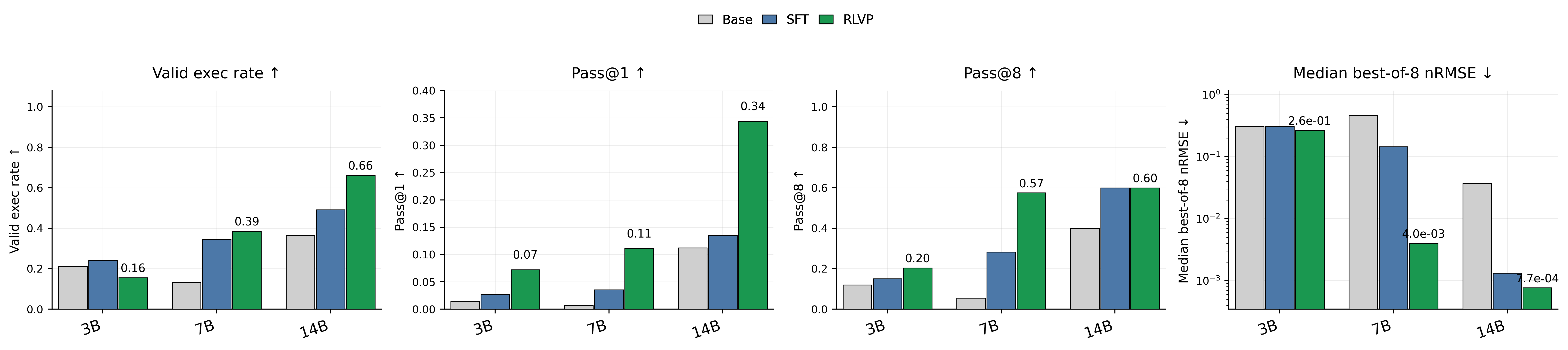
RLVP improves on heat, 2D advection, advection–reaction–diffusion, and Cahn–Hilliard. Advection–diffusion, Darcy–reaction, and KdV remain challenging.
Zero-shot transfer to 3D PDEs
No 3D examples are used during SFT or RL. We evaluate the frozen 14B model trained with the accuracy-only reward on five 3D problems, using prompts that do not specify a numerical method. These results suggest some transfer of numerical methods to 3D problems.
| 3D PDE | Base 14B | RLVP 14B | ||
|---|---|---|---|---|
| Pass@1 | Pass@8 | Pass@1 | Pass@8 | |
| Advection | 0.0% | 0.0% | 21.9% | 89.7% |
| Heat | 21.9% | 89.7% | 50.0% | 99.9% |
| Fisher–KPP | 28.1% | 95.3% | 45.3% | 99.7% |
| Gray–Scott | 28.1% | 95.3% | 87.5% | 100.0% |
| Acoustic wave | 0.0% | 0.0% | 2.1% | 16.7% |
32 generated programs per prompt, six hidden cases per PDE, and 24 × 24 × 24 grids. Pass@8 is estimated combinatorially from the 32 samples.
BibTeX
@inproceedings{cai2026rlvp,
  title     = {Reinforcement Learning with Verifiable Physics:
               Post-training LLMs with Continuous Rewards},
  author    = {Cai, Pengfei and Utkarsh, Utkarsh and Edelman, Alan
               and Rackauckas, Christopher Vincent
               and Gomez-Bombarelli, Rafael},
  booktitle = {Advances in Neural Information Processing Systems},
  year      = {2026},
  url       = {https://arxiv.org/abs/2607.10474}
}